Stateless audio synthesis intro

Balance uses a tool called minimal_gl.

minimal_gl makes it really easy to get started. You just have to write two OpenGL shaders: one for visuals, and one for audio. minimal_gl does the rest (with support from crinkler and shader minifier).

minimal_gl is really minimal, which is great because it saves bytes. It’s so minimal that the two shaders you provide have to be pure, stateless functions. This means that the audio function takes a time argument, and from only that information it has to compute a sample value.

This is a challenge!

Before diving into the individual instruments, let’s look at some of the implications of stateless audio synthesis.

Audio synthesis in 4k intros is a well-explored area. Typically intros use size-optimized versions of “normal” synthesis, e.g. subtractive, additive, or FM synthesis plus various effects like reverbs, filters, and so on.

Most effects are built on delay lines, which are stateful. This rules out delays, reverbs, choruses, compressors, and so on.

IIR filters are also stateful and therefore impossible in minimal_gl, ruling out most common filters, upsampling/downsampling, and the whole field of subtractive synthesis.

We’re basically left with additive synthesis, FIR filters and FM synthesis.

But there are also blessings in this approach:

• Statelessness reduces code complexity - you can express a lot with a few characters
• The constraints of the typical synthesizer architecture fall away: we can design instruments that would be unreasonable to consider in a size-optimized stateful architecture
• Shader hot reloading enables very fast iteration

In fact, the above three bullets are a sum-greater-than-its-parts situation. It is very productive and fun to work this way.

Let’s put these ideas into practice by designing a few instruments from scratch, starting with the backbone of any track: the kick drum.

Kick Drums

First, here are the two kick drum sounds we’re going to create.

Decaying Sine

Let’s start with a 40Hz sine wave, with a decay.

vec2 dirtykick2(float t) {
    float phase = 40.0 * t;
    float decay = exp(-t * 6.0);
  
    vec2 V = vec2(sin(TAU * phase) * decay);
    return V;
}

A couple of notes:

• t is the time in seconds
• TAU is defined externally to be 2 times pi, approximately 6.2830…
• We return a vec2 because our audio is stereo. The x and y components of the vector map to the left and right channels respectively, although we are not using this yet.

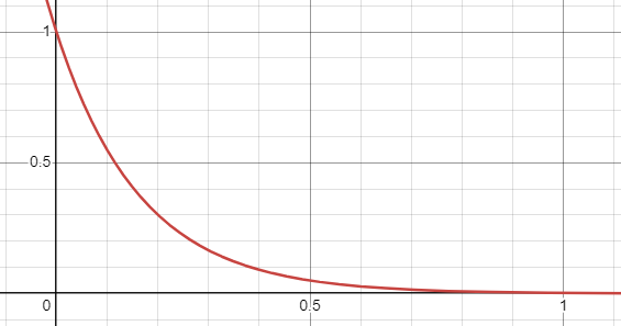
exp(-t * 6.) is an exponential decay function that starts at 1 and goes to 0 in a way that is very natural sounding.

The first second of the curve looks like this.

Integrated exponential frequency glide

Typically we like our kick drums to start at a higher frequency, and then glide to a lower one. Here I’ve chosen to glide from 160Hz to our 40Hz base note.

We can reuse the idea of the exp function to change our frequency, e.g. like this:

freq = 40.0 + 120.0*exp(-t * 10.0)

That’s great, but we run into a problem. We need phase, not freq! We can’t immediately just compute phase from freq. That would require knowledge about how freq changed over time - in fact, it requires that we integrate freq over time, which gives us exactly phase!

Fortunately the integration is pretty easy. Generalizing our frequency sweep expression to f0*exp(-t * kappa) where f0 is the value at t=0 and kappa is the time constant, we get

float integrate_exp(float t, float f0, float kappa) {
    return (f0 / kappa) * (1.0 - exp(-kappa * t));
}

With this, we can update our code snippet:

    float phase = 40.0 * t;
    phase += integrate_exp(t, 120.0, 10.0);

If we could have used state, we could have kept phase in an accumulating variable, and updated it according to freq every sample, and that would have worked. Something like phase += freq(t) / SAMPLES_PER_SEC - which happens to be a simple numerical integrator!

Noise attack

Now that we have the tonal body of the kick, we can give it more impact with a short burst of noise at the start of the sound:

V += hash12(t) * exp(-t * 50.);

hash12 is a function that returns white noise based on one input parameter (time).

Note that hash12 returns a vec2 with different noise for left and right channels, so our kick is now stereo!

Making it dirty with phase noise

The sound is clean but sterile. To give it character, we’ll randomize its phase slightly over time.

    phase += hash11(t) * 0.035 * exp(-t * 10.0);

The constants here can be tweaked.

Tying together with tanh

If you listen closely, the elements of our sound are a bit disjoint, lacking “togetherness”. The are a number of ways to adress this, but the simplest and easiest way in this context is to distort with tanh.

While we’re at it, I’ll also pull the stereo channels closer together with stereowidth. This leaves more room for other instruments in the stereo space.

This is our completed dirty kick instrument.

vec2 dirtykick2(float t) {
    float phase = 40.0 * t;
    phase += integrate_exp(t, 120.0, 10.0);
    phase += hash11(t) * 0.035 * exp(-t * 10.0);
    float decay = exp(-t * 6.);
  
    vec2 V = vec2(sin(TAU * phase) * decay);
    V += hash12(t) * exp(-t * 50.);
    V = tanh(V * 2.0);
    V = stereowidth(V, 0.75);
    return V;
}

Alternate kick

Our alternate kick is very similar in terms of code. I have removed the phase noise, used the full stereo width, and I’ve added a signal multiplier using abs and sin which gives it a little bounce in the low end.

vec2 kick(float t) {
    float phase = 40.0 * t;
    phase += integrate_exp(t, 120.0, 10.0);
    float decay = exp(-t * 6.);
  
    vec2 V = vec2(sin(TAU * phase) * decay);
    V += hash12(t) * exp(-t * 50.);
    V = tanh(V * 2.0);
    V *= abs(sin(t * 15.));
    return V;
}

It might have been better to use cos with abs in the second to last line. sin starts at zero, which kills the attack of the sound.

With a couple of solid kick variations in place, let’s move on to brighter percussive elements.

Hihat

One common recipe for hihat: white noise → highpass filter → decayed volume.

Here’s what that will sound like for us.

Decayed noise

Let’s start with just some white noise with a decaying volume envelope.

vec2 hihat(float t) {
    vec2 V = vec2(0.0);
    V += hash12(t + 11.89);
    V *= vec2(exp(-t * 12));
    return V * 0.3;
}

The raw noise gives us energy, but it needs spectral shaping to become a hihat. Since we can’t use IIR filters, we’ll compensate with FIR.

Stateless filtering: FIR

Let’s filter our noise.

Most filters in typical synths are IIR filters. IIR filters can sound great, are cheap to compute - but they require state.

Is there a way to filter when you only know the current time?

Turns out it’s possible with FIR filters!

There is a lot of theory to explain here, much more than I can go into. Rather than considering only the current filter input and the filter state for every sample, FIR filters consider the last N samples (say N = 65), and multiplies (convolves) them with a filter kernel.

And - if you’ve implemented FIR filters before, now you’re asking: where will we store the 65 preceding samples? Where will we store the FIR filter kernel?

Answer: We don’t! We just recompute them every sample!

So for each sample we compute the previous 65 sample values, and the 65 values in our FIR kernel, and convolve them!

Easy? Yes!

Cheap? No! This is quite expensive in terms of GPU cycles.

Here are the functions we need to generate highpass, lowpass and resonance kernels, with N values and cutoff at fc .

float sinc(float x) {
    return abs(x) < 1e-7 ? 1.0 : sin(x) / x;
}

float blackman(int k, int N) {
    float t = TAU * float(k) / (float(N) - 1.0);
    return 0.42 - 0.5 * cos(t) + 0.08 * cos(2.0 * t);
}

float lp_tap(int k, int N, float fc) {
    float m = 0.5 * (N - 1), a = fc / SAMPLES_PER_SEC, x = float(k) - m;
    float hlp = 2.0 * a * sinc(TAU * a * x);
    return hlp;
}
  
float hp_tap(int k, int N, float fc) {
    // Spectral inversion
    return ((k == ((N - 1) / 2)) ? 1.0 : 0.0) - lp_tap(k, N, fc);
}
 
float res_tap(int k, int N, float fc, float g) {
    float m = 0.5 * (N - 1), wc = TAU * fc / SAMPLES_PER_SEC, x = float(k) - m;
    return g * cos(wc * x);
}

A few notes:

• This implements a basic method for FIR filter design called windowed-sinc FIR filter design. You can google or ChatGPT it.
• The Blackman window is interesting because it is simple to compute, and directly gives attenuation proportional to the length of the kernel. (On a personal note I find the tradeoff between implementation length and attenuation in window functions super fascinating!)

We replace our simple hash call with a filtered hash:

vec2 hihat(float t) {
    vec2 V = vec2(0.0);
  
    const int N = 65;
    repeat(n, N)
    {
        float tap = hp_tap(n, N, 4000.0) * blackman(n, N);
        V += hash12(t + 11.89 + float(n) / SAMPLES_PER_SEC) * vec2(tap);
    }
  
    V *= vec2(exp(-t * 12));
    return V * 0.3;
}

Notes:

• For N = 65 we get approximately 24dB rolloff per octave.
• hash12(t + 11.89 + float(n) / SAMPLES_PER_SEC)
  • I add 11.89 because the hash12 function I used is not very white around 0
  • float(n) / SAMPLES_PER_SEC is the sample time offset we use to sample the last 65 samples of the hash12 function

The FIR approach works beautifully but comes at a cost. Each sample re-evaluates dozens of taps, so it’s worth thinking about efficiency.

Optimizing with early outs

This hihat is expensive to compute, so we might think about how to help out the GPU a bit.

Consider that there is no concept of note on and note off here. Only time t. And from the point of view of the hihat2 function, we don’t have any guarantees about what values t will take.

So a good idea is to check the t argument, and skip the sound computation if we know we are not generating sound! This can be done with a couple of simple lines as the first thing in the function:

vec2 hihat(float t) {
    if (t < 0.0 || t > 0.35)
        return vec2(0.);
[...]

t < 0.0 is hopefully an obvious check. t > 0.35 is found by trial and error.

Here’s the hihat loop:

Snare

YouTube has a bunch of people who are very happy to talk about instrument design in great detail.

For example, here are two examples of people talking about designing snare drums:

• How To Synthesize Snare Drums
• How to make a Snare Drum with synthesis, 3 minute tutorial

Following the example in the first video, this is what we get:

Click

Let’s start with a very short burst of initial high-pass filtered noise for an attack.

vec2 snare2(float t, float free_time) {
    vec2 click = vec2(0.0);
    const int N = 65;
    repeat(n, N)
    {
        float tap = hp_tap(n, N, 1000.0) * blackman(n, N);
        click += hash12(free_time + float(n) / SAMPLES_PER_SEC) * vec2(tap);
    }
    click *= linearenvwithhold(t, 0.003, 0.005, 0.001);
    click = stereowidth(click, 0.5);
  
    return click;
}

We could consider adding an early out check for the click. One way to do that could be to compute the envelope value first, and skip the filtering if the envelope is zero.

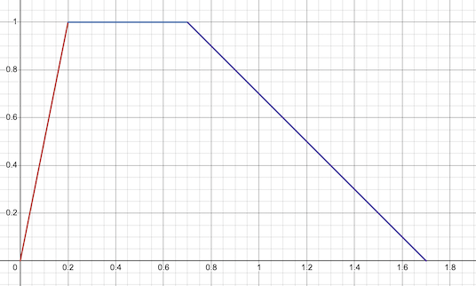
The envelope is a very simple linear envelope. Here is an example with attack = 0.2, hold = 0.5 and release = 1.0.

Note I am passing both t and free_time parameter to snare2. t is still the primary controlling time parameter. free_time is a longer-period time I use as noise seed. This makes the drum sound slightly different every hit. Totally optional.

With the initial click defined, we can now give the snare its tonal center: the resonating drum body.

Body

The body is a frequency-decaying sine (175Hz → 160Hz) with distortion.

Here is the sine alone:

And distorted with the click:

vec2 snare2(float t, float free_time) {
    [click...] 

    float bodyphase = TAU * (160.f * t + integrate_exp(t, 40.f, 15.0f));
    vec2 body = vec2(0.4 * sin(bodyphase));
    body *= linearenvwithhold(t, 0.010, 0.020, 0.100);
    vec2 body_and_click_distorted = tanh(click + body * 3.0);

    return body_and_click_distorted;
}

The body is mono.

Noise

Now let’s add the tail noise, which is white noise with a resonant FIR filter around 5000Hz.

Here is the noise alone:

Here is the noise with the click and the body:

    vec2 noise = vec2(0.0);
    const int N2 = 21;
    repeat(n, N2)
    {
        float tap = res_tap(n, N, 5000.0, 0.9) * blackman(n, N);
        noise += hash12(free_time + float(n) / SAMPLES_PER_SEC) * vec2(tap);
    }
    noise *= linearenvexp(t, 0.035, 13.0);
    noise = stereowidth(noise, 0.3);

I only use 21 taps for the resonant peak filter, which gives the resonance a wide spectrum.

Additive tonal ring

Real snares often have metallic overtones that linger after the hit. We can model that with an additive bell-like component.

Here it is isolated:

Here it is in combination with other parts, which forms our complete drum:

    vec2 tonal_ring = vec2(0.);
    repeat(i, 12)
    {
        vec3 r = (hash13(float(i + 16.7))) * 0.5 + 0.5;
        float freq = 160. + 40. * r.x;
        float ampl = exp(-3.0 * r.z);
        float phase = TAU * r.y;
        tonal_ring += tanh(vec2(ampl * vec2(cos(phase + TAU * freq * t), sin(phase + TAU * freq * t))) * 2.0);
    }
    tonal_ring *= linearenvexp(t - 0.015, 0.010, 10.0);
    tonal_ring = stereowidth(tonal_ring, 0.3);
  
    return tanh(body_and_click_distorted * 0.3 + noise * 0.2 + tonal_ring * 0.07) * 5.0;

Okay, now we’re doing something really additive!

We’re adding 12 partials, indexed by i.

For each partial I make a random vec3 from hash13. Because I only use i as a seed, not time, this random vector will be the same for the partial for all samples, so we can use this to randomize partials: I use r.x to select a random frequency between 160Hz and 200Hz, r.z to vary the amplitude and r.y to vary phase. Then I add a little stereo with cos/sin, and distort the individual partials with tanh.

Then we just sum the 12 partials, run it through an envelope and reduce the stereo width.

We will be reusing this additive technique for the pad and the wah-sound.

Here’s the full percussion loop:

Pad

The pad is purely additive. Here’s what the final result sounds like:

Additive harmonics

We’ll start with a very simple sound with 30 harmonics.

vec2 pad(float t, float note_freq) {
    vec2 V = vec2(0.0);
  
    const int NUM_MODES = 30;
    repeat(mode, NUM_MODES)
    {
        float mode_freq = note_freq * (mode + 1.0);
  
        float mode_magnitude = pow(2.0,  (1.5 + 3.0 * mode / float(NUM_MODES)));
        mode_magnitude *= 1.0 / pow((mode_freq / note_freq), 1.5);
  
        V += mode_magnitude * sin(TAU * mode_freq * t);
    }

    float env = linearenvwithhold(t, 2.0, 16.0, 2.0);
    return V * 0.04;
}

I am using the term mode in the code instead of harmonic or partial. This originates from modes of a distribution. Maybe you’ll be able to see why in the Paderizing section.

First, I compute the harmonic frequency mode_freq as a partial frequency (a multiple of base note_freq).

Second, I compute a magnitude for the mode. This looks a bit complex - this is where I ended up after iterations on getting it to sound good, so this is just artistic choice. Generally partial magnitude should be approximately 1.0 / partial, or the sound will be very bright/harsh.

Finally, we sum the modes together and apply an envelope.

Additive harmonics with evolution

This sounds very static so far. Let’s evolve the mode_magnitude over time with sines.

vec2 pad(float t, float note_freq) {
    vec2 V = vec2(0.0);
 
    const int NUM_MODES = 30;
    repeat(mode, NUM_MODES)
    {
        vec3 mode_r = hash13(mode * 13.1 + 9.9128783);

        float mode_freq = note_freq * (mode + 1.0);

        float mode_magnitude = pow(2.0,  (1.5 + 3.0 * mode / float(NUM_MODES)) * mode_r.x * sin(TAU * (0.02 + 0.13 * mode_r.y) * t + mode_r.z));
        mode_magnitude *= 1.0 / pow((mode_freq / note_freq), 1.5);
  
        V += mode_magnitude * sin(TAU * mode_freq * t);
    }

    float env = linearenvwithhold(t, 2.0, 16.0, 2.0);
    return V * 0.04;
}

I am introducing the mode_r variable here, which is a random value for each mode that is consistent across samples (it only depends on the mode index for seed).

We use this to apply a sine evolution to the mode magnitude, with mode_r.x, mode_r.y and mode_r.z influencing magnitude, frequency and phase respectively.

Paderizing

To widen and soften the sound, we’ll spread each harmonic across many slightly detuned and panned voices. This is a classic pad technique we can reproduce statelessly.

To start, let’s try with just 1 voice per harmonic (NUM_SINES_PER_MODE = 1).

Here are all 19 voices.

vec2 pad(float t, float note_freq) {
    vec2 V = vec2(0.0);
  
    const int NUM_MODES = 30;
    repeat(mode, NUM_MODES)
    {
        vec3 mode_r = hash13(mode * 13.1 + 9.9128783);
  
        float mode_freq = note_freq * (mode + 1.0);
  
        float mode_magnitude = pow(2.0,  (1.5 + 3.0 * mode / float(NUM_MODES)) * mode_r.x * sin(TAU * (0.02 + 0.13 * mode_r.y) * t + mode_r.z));
        mode_magnitude *= 1.0 / pow((mode_freq / note_freq), 1.5);
  
        float mode_rel_oct = log(mode_freq / note_freq);
  
        const int NUM_SINES_PER_MODE = 19;
        repeat(i, NUM_SINES_PER_MODE)
        {
            vec3 r = hash13(mode * 1.1 + 11.9128783 + i * 1.9);
  
            float freq = mode_freq * pow(2.0, sqrt(sqrt(mode_rel_oct + 2.0)) * 0.02 * r.x);
            float O = mode_magnitude * sin(TAU * freq * t + r.z * TAU);
  
            V += O * pan(r.y * 0.5 + 0.5, -4.5);
        }
    }
  
    float env = linearenvwithhold(t, 2.0, 16.0, 2.0);

    return V * 0.04;
}

I’ve replaced the single sine per harmonic with a loop. Each sine has an r random variable (depending on both mode and sine index), that we use to find a random frequency around mode_freq, to offset the sine phase, and to randomly pan.

Compression / Sidechaining

We can’t use compressors because they are stateful. But we can approximate a compressor effect by manually computing an envelope for an instrument (or a group of instruments), and using that to reduce the volume of other instruments. I noticed that the pad was clashing a bit with the percussion, so I decided to sidechain the pad’s volume based on the percussion envelope.

This gives a nice pumping effect, which I decided to leave in for the beginning before the drums start.

    float percsidechain =
        1.0 * linearenvwithhold((beat.y - 2.5) * B2T - 0.050, 0.050, 0.250, 0.100)
      + 0.8 * linearenvwithhold((beat.y - 0.0) * B2T - 0.000, 0.010, 0.140, 0.100)
      + 0.7 * linearenvwithhold((beat.y - 1.0) * B2T - 0.000, 0.010, 0.100, 0.100);
    percsidechain = 1.0 - tanh(percsidechain * 1.5);

As you can see, I am just manually estimating the percussion envelope by summing three linear envelopes, one per drum hit. As an alternative, instead of centralizing the percussion envelope computation here, I could have computed it in the drum functions and returned the value. That would have been more general, and easier to play with.

Wah

Okay, last instrument, some simplified voice synthesis!

In our rough model, there are two components to making a vowel sound.

1. An underlying sound produced by the vocal cords
2. The formants that shape the sound, based on resonances and filters in the vocal tract

Formants

According to the dictionary, a formant is

“each of several prominent bands of frequency that determine the phonetic quality of a vowel”

I used this table for formant data: https://www.classes.cs.uchicago.edu/archive/1999/spring/CS295/Computing_Resources/Csound/CsManual3.48b1.HTML/Appendices/table3.html

Each formant has a center resonant frequency (Hz), a resonant amplitude (dB) and width of resonant peak (Hz).

I am using the tenor “a” and the tenor “o” from that page. I’ve created this table, manually converting dB to gains for the two formant sets.

const vec3 formant_table[10] = vec3[](
        // tenor "a"
        vec3(650, 1.00, 80),
        vec3(1080, 0.50, 90),
        vec3(2650, 0.45, 120),
        vec3(2900, 0.40, 130),
        vec3(3250, 0.08, 140),
        
        // tenor "o"
        vec3(400, 1.00, 40),
        vec3(800, 0.32, 80),
        vec3(2600, 0.25, 100),
        vec3(2800, 0.25, 120),
        vec3(3000, 0.05, 120)
    );

Formant function

Since formants shape an underlying sound, basically describing the resonant frequencies, we need to be able to determine how strongly a specific frequency resonates gives a formant.

For that I use this function:

float filterformant(float freq, vec3 formant) {
    float f = formant.x;
    float gain = formant.y;
    float bw = formant.z * 2.0;
    float bw_squared = bw * bw;
  
    float V = exp(-pow(freq - f, 2.0) / (2.0 * bw_squared));
    V *= gain;
    return V;
}

We unpack the formant information in the vector, and then evaluate a Gaussian function (which gives a nice soft curve) at the given input frequency. The Gaussion curve is centered at the formant frequency, has a standard deviation matching the formant bandwidth, and the height of the formant amplitude.

There is nothing magical about the Gaussion. Any other curve with the appropriate properties will do. A triangle curve is another perfectly valid way to do it.

Underlying sound

Let’s produce the underlying sound:

vec2 pad3voice(float t, float barnum, float note_freq) {
    float barpos = t * T2B;
  
    vec2 V = vec2(0.0);
  
    const int NUM_MODES = 30;
    repeat(mode, NUM_MODES)
    {
        vec3 mode_r = hash13(mode * 13.1 + 9.9128783 + barnum * 0.1432);
  
        float mode_freq = note_freq * (mode + 1.0);
  
        float mode_magnitude = pow(2.0, 1.07 * mode_r.x * sin(TAU * (0.02 + 0.13 * mode_r.y) * t + mode_r.z));
        mode_magnitude *= 1.0 / pow((mode_freq / note_freq), 1.5);
  
        float rel_oct = log(mode_freq / note_freq);
  
        const int NUM_SINES_PER_MODE = 19 * 2;
        repeat(i, NUM_SINES_PER_MODE + int(mode))
        {
            vec3 r = hash13(mode * 1.1 + 11.9128783 + i * 1.9 + barnum * 0.1432);
  
            float freq = mode_freq * pow(2.0, sqrt(sqrt(rel_oct + 2.0)) * 0.027 * r.x);
  
            float env = linearenvwithhold(barpos, 0.15 + abs(r.x) * 0.01, 0.3 + abs(r.y) * 0.003, 0.5 + abs(r.z) * 0.05);
  
            float O = mode_magnitude * env * sin(TAU * freq * t + r.z * TAU);
            V += O * pan(step(r.y, 0.0), -4.5);
        }
    }
  
    V = stereowidth(V, 0.6);
    return V * 0.4;
}

This is a variant of the pad. The main differences are:

• Added a barnum parameter to randomize the sound a bit, so each section of the wah sound varies slightly
• Increased the number of sines per mode to get a richer sound
• Added an envelope per sine with some randomization to model a human choir better
• Changed some constants to get a slightly different timbre that sounded more like a voice

These were all trial and error differences with the goal of making it sound more human.

Formant shaping

Now let’s use the tenor “o” formants to shape the sound.

This means evaluating the frequency of each sine in the underlying sound with respect to the resonant formants, multiplying the sine magnitude with the formant response.

vec2 pad3voice(float t, float barnum, float note_freq) {
    float barpos = t * T2B;
  
    vec2 V = vec2(0.0);
  
    const int NUM_MODES = 30;
    repeat(mode, NUM_MODES)
    {
        vec3 mode_r = hash13(mode * 13.1 + 9.9128783 + barnum * 0.1432);
  
        float mode_freq = note_freq * (mode + 1.0);
  
        float mode_magnitude = pow(2.0, 1.07 * mode_r.x * sin(TAU * (0.02 + 0.13 * mode_r.y) * t + mode_r.z));
        mode_magnitude *= 1.0 / pow((mode_freq / note_freq), 1.5);
  
        float rel_oct = log(mode_freq / note_freq);
  
        const int NUM_SINES_PER_MODE = 19 * 2;
        repeat(i, NUM_SINES_PER_MODE + int(mode))
        {
            vec3 r = hash13(mode * 1.1 + 11.9128783 + i * 1.9 + barnum * 0.1432);
  
            float freq = mode_freq * pow(2.0, sqrt(sqrt(rel_oct + 2.0)) * 0.027 * r.x);

            float formant = 0.0;
            repeat(n, 5)
            {
                formant = max(formant, filterformant(freq, formant_table[n+5]));
            }
  
            float env = linearenvwithhold(barpos, 0.15 + abs(r.x) * 0.01, 0.3 + abs(r.y) * 0.003, 0.5 + abs(r.z) * 0.05);
  
            float O = mode_magnitude * env * formant * sin(TAU * freq * t + r.z * TAU);
            V += O * pan(step(r.y, 0.0), -4.5);
        }
    }
  
    V = stereowidth(V, 0.6);
    return V * 0.4;
}

Formant morphing

Applying only a single tenor “o” formant sounds robotic. Human voices clearly don’t work this way!

Let’s add a morph from tenor “o” to tenor “a” in the sound.

Here I replace the four formant lines with this loop:

            float formant_glide = smoothstep(0.0 - abs(r.x) * 0.05, 0.5 + r.y * 0.03, barpos);
  
            float formant = 0.0;
            repeat(n, 5)
            {
                formant = max(formant, filterformant(freq, mix(formant_table[n + 5], formant_table[n], formant_glide)));
            }

Conclusion

We got far without any state at all! We used analytical integration, FIR filtering, and additive synthesis to create a full percussion set, a pad, and a wah-like voice synthesis instrument.

This approach feels very liberating. Very creative. Changes are quick to make. I don’t need on a large library of stateful DSP building blocks.

It feels close to visual shader programming because of the short feedback loop; flow is easy.

I am quite optimistic about this direction. I have many more ideas to explore. We didn’t even get into FM synthesis, and I can also see how a more structured approach to instrument implementation inspired by something like Native Instruments Razor could be an interesting direction.

That’s all, thank you for reading this far.